British Columbia groundfish

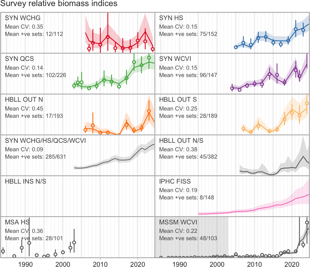
Example relative biomass index trends from trawl and longline surveys for Petrale Sole. Dots represent design-based mean estimates of relative biomass and vertical lines around the dots represent 95% bootstrap confidence intervals. Time series with a solid trend line and shaded ribbon for 95% confidence intervals represent an index that has been standardized with a spatiotemporal model (see Appendix A in DFO 2022a). Spatiotemporal-model-based indices are omitted for a survey-species combination if fewer than 5% of sets contained the species or if no models converged.

‘Mean CV’ is the mean of the annual coefficients of variation (CVs), and ‘Mean +ve sets’ indicates the ratio of the mean number (across the years) of sets that captured the species of interest to the mean number of sets. All vertical axes are scaled between zero and the maximum upper confidence interval value for that survey. When both types of indices are shown, they are scaled to have the same geometric mean and the axes are set to encompass the model-based confidence intervals. For the MSSM WCVI, years before 2003 are shaded grey to indicate that catches are considered less reliable than modern data. For the HBLL OUT, HBLL INS, and IPHC FISS the values are abundance rather than biomass. Also included are coastwide or survey-wide indices for SYN WCHG/HS/QCS/WCVI, HBLL OUT N/S, and HBLL INS N/S.

SYN WCHG

West Coast Haida Gwaii Synoptic Bottom Trawl

SYN HS

Hecate Strait Synoptic Bottom Trawl

SYN QCS

Queen Charlotte Sound Synoptic Bottom Trawl

SYN WCVI

West Coast Vancouver Island Synoptic Bottom Trawl

HBLL OUT N

Hard Bottom Longline Outside North

HBLL OUT S

Hard Bottom Longline Outside South

HBLL INS N

Hard Bottom Longline Inside North

HBLL INS S

Hard Bottom Longline Inside South

IPHC FISS

International Pacific Halibut Commission Fishery-Independent Setline Survey

MSA HS

Hecate Strait Multispecies Assemblage Bottom Trawl

MSSM WCVI

West Coast Vancouver Island Multispecies Small-mesh Bottom Trawl

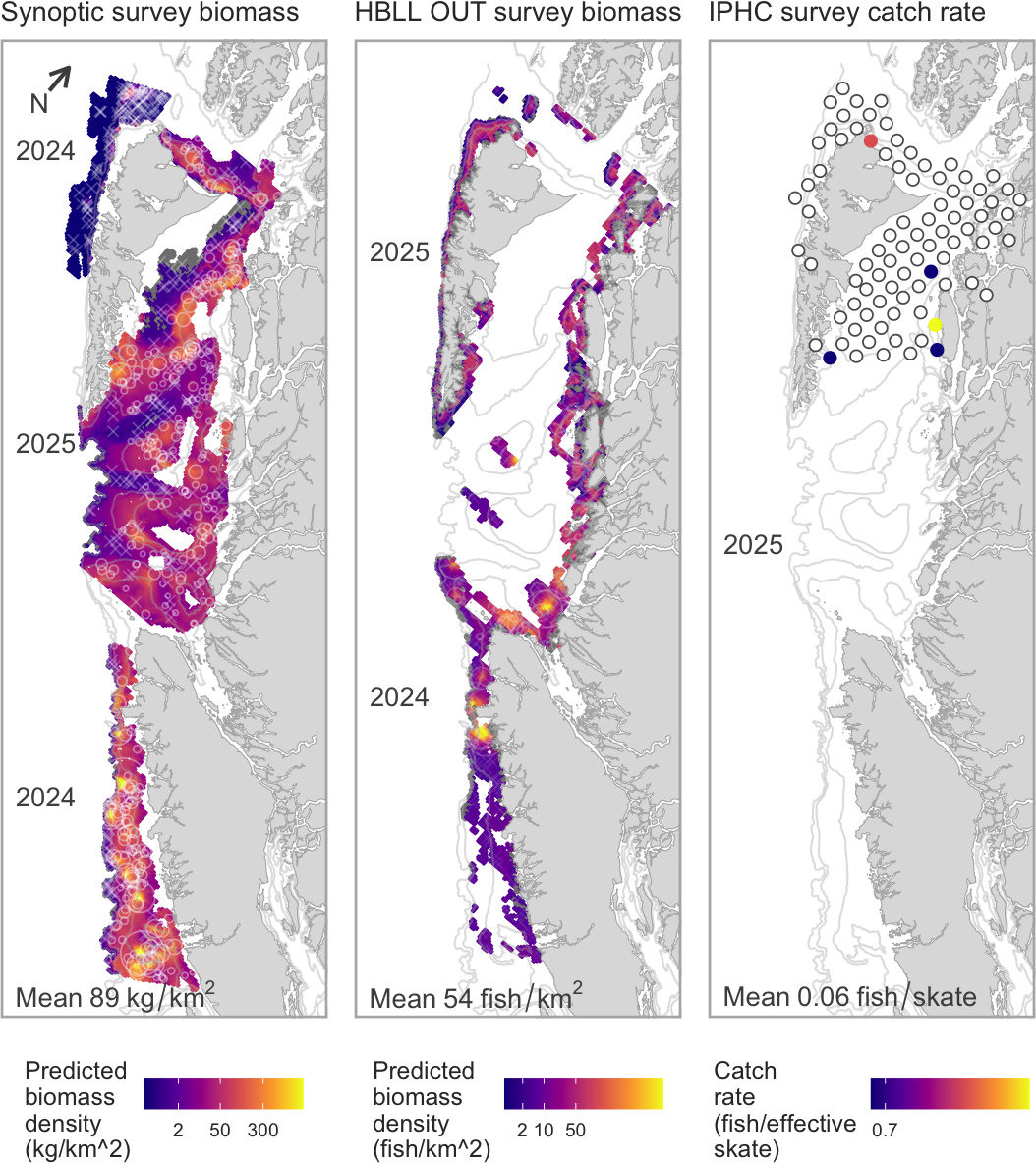
Example maps of relative biomass (or catch rate) from trawl and longline surveys from the latest available years of each survey for Petrale Sole. Shown are the synoptic trawl surveys (left), the outside hard bottom longline (HBLL OUT) surveys (middle), and the IPHC FISS (right). Individual sets are shown in the two left panels as faint crosses (if the species was not caught in that set), or circles with the area of the circle proportional to the species density from the set.

Colour shading (except for the IPHC survey) indicates predictions from a spatial model that includes depth and depth squared as predictors as well as spatial random effects (Appendix E in Anderson et al. 2019). The colour scale is fourth-root transformed to render a visual pattern similar to a log transformation without overemphasizing differences close to zero. The colour scale ranges from zero to the highest value within each map, and dark grey indicates regions where models could not be fit.

The synoptic and HBLL maps show predicted biomass density throughout the survey domain. The IPHC map shows the raw unmodelled data for fixed station locations—stations without any observations for a given species are shown as empty circles. Years on the left side of each plot indicate the year of the respective survey. Surveys (except IPHC) in which less than 2% of the sets contained the species are not modeled and are shown with raw data only.

Mean values shown at the bottom are the mean fish density values from the raw data for the entire coast for the indicated years; for the IPHC data the units are fish per effective skate, where an effective skate represents 100 circle hooks with 18-foot spacing (Appendix G in Anderson et al. 2019). Note that the coast has been rotated 40° to fit all the maps in the available space. Depth contours are shown at 100 m, 200 m, and 500 m.

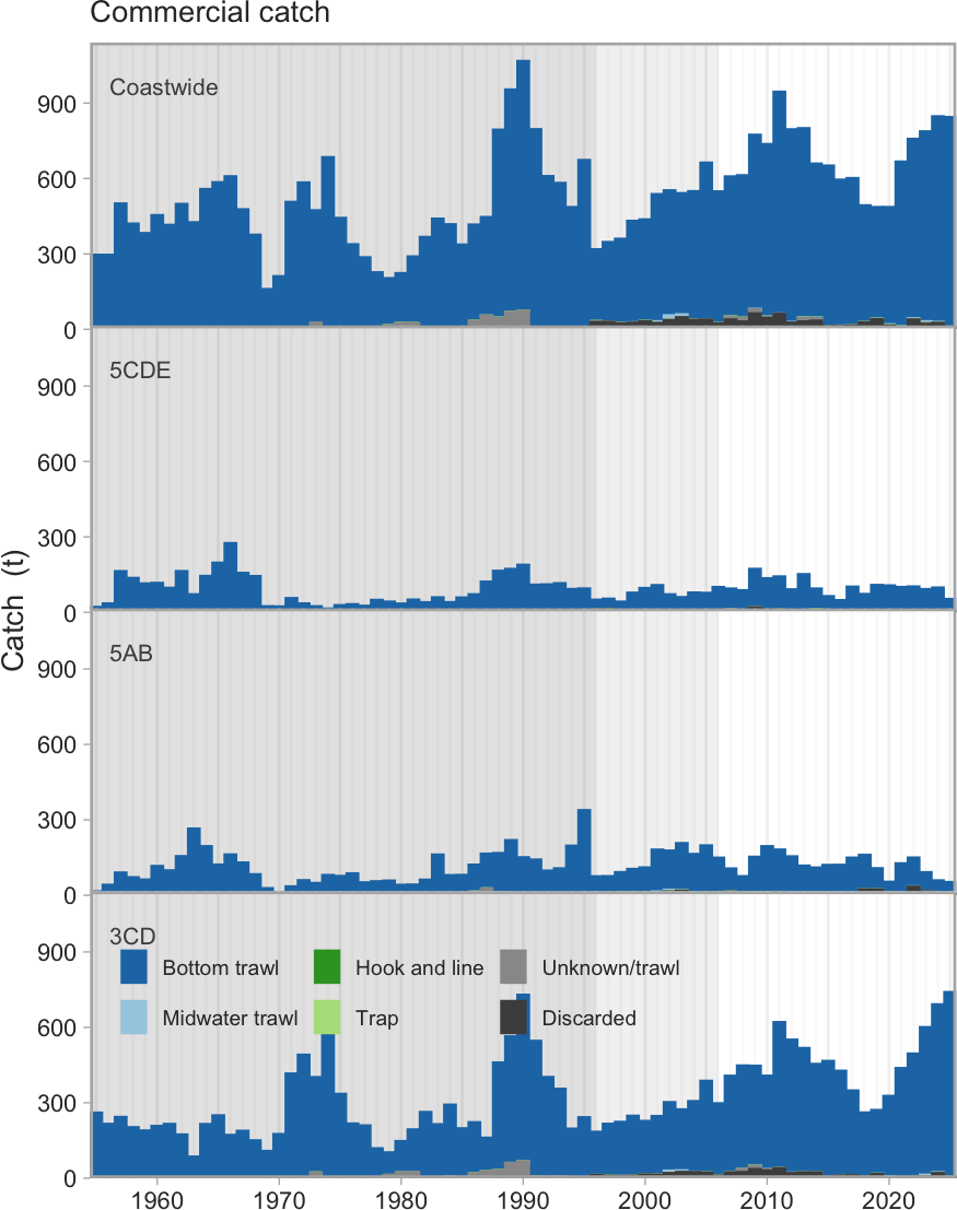
Example commercial fishery catch plots for Petrale Sole. Catch from various gear types is indicated by colour shading. Catch is calculated as the summed weight of landings aggregated by year. Discards include reported discard weights from all fisheries combined; however, bottom trawl discards are considered less reliable prior to 100% observer coverage in 1996 and trap, hook and line, midwater trawl, and Strait of Georgia bottom trawl discards are less reliable prior to fisheries integration in 2006 and are therefore not included.

Catch data prior to 1996 and 2006 are shaded grey to indicate they are considered less reliable than more recent data. Catch estimates from the bottom and midwater trawl fleets operating in outside waters are less certain before the introduction of an at-sea observer program in 1996. Similarly, catch estimates from non-trawl sectors (longline and trap) are less certain prior to the implementation of an at-sea electronic monitoring (EM) program in 2006. The at-sea observer program for the trawl fleet was discontinued in early 2020 due to COVID-19. Since then, the trawl fleet has been monitored using EM systems. EM systems are supplemented by port-based biological sampling for some species. Management areas, as indicated in the top left corner of each panel, are shown in Figure 2.

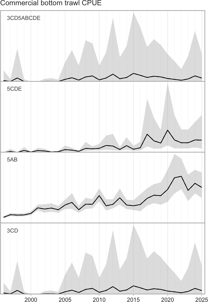
Example commercial bottom trawl catch per unit effort (CPUE) trends, with effort as hours trawled, for Petrale Sole. Commercial CPUE has been standardized with a spatiotemporal model. The line and shaded region represent the mean and 95% confidence interval. Standardized time series are scaled to have the same maximum 95% confidence interval. Management areas, as indicated in the top left corner of each panel, are shown in Figure 2.

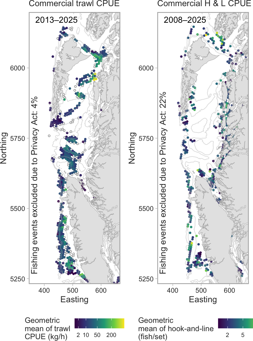
Example commercial trawl and commercial hook-and-line catch-per-unit-effort maps for Pacific Cod (note this figure is not Petrale Sole because the hook-and-line panel is mostly blank for Petrale Sole). Lighter shading indicates higher levels of a geometric mean of catch per unit effort in a given hexagonal cell. The colour scale is fourth-root transformed to render a visual pattern similar to a log transformation without overemphasizing differences close to zero. Cells are 7 km wide and are only shown in cases where there are at least 3 unique vessels in a given cell to meet privacy requirements.

For bottom trawl, catch per unit effort is calculated as the weight of catch (landings plus discards) divided by hours fished for all positive tows from the groundfish trawl sector. Trawl data are shown from 2013 onwards after the trawl footprint was [ecosystem-based trawling boundaries were established; Wallace et al. (2015)]. Trawl data from 2007–2012 are indicated as outlined light grey hexagons to illustrate fishing prior to the frozen footprint. For hook and line, catch per unit effort is shown as the number of fish recorded as landed or discarded per set. Hook-and-line data are shown from 2008 onwards. Including as many years of data as possible reduces the number of discarded fishing events when implementing the 3-vessel privacy requirement.

Note that the coast has been rotated 40° to fit all the maps in the available space. Depth contours are shown at 100 m, 200 m, and 500 m.

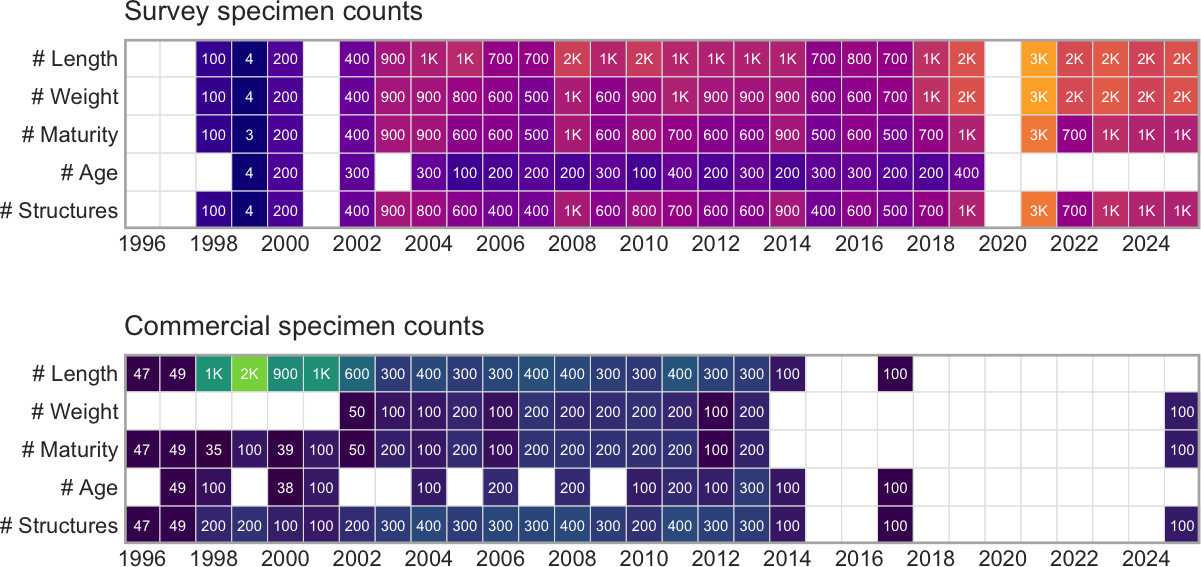
Example specimen-availability plot for Petrale Sole. Shown are the number of available fish specimens that have had their length measured, have been weighed, had their maturity assessed, had their age assessed, and for which ageing structures are available for ageing.

Data are shown across all surveys (not just surveys shown elsewhere in the synopsis; top panel) and across all commercial fleets (bottom panel). Blank panels indicate year-measurement combinations without any data. Shading of these cells reflects the relative number of specimens available with the actual number of specimens indicated in the cells to the nearest round number.

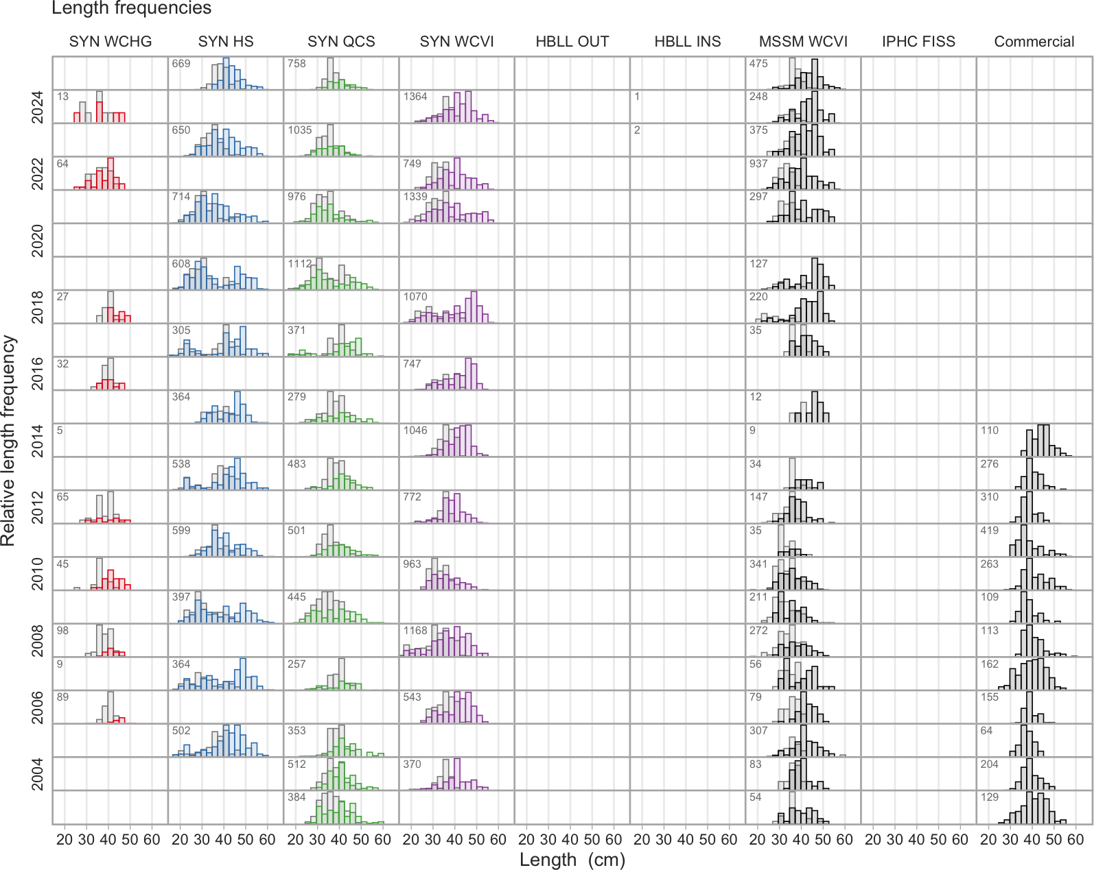
Example length-frequency plot for Petrale Sole. Female fish are shown as coloured (or black) bars and male fish are shown behind as light grey bars. The total number of fish measured for a given survey and year are indicated in the top left corner of each panel. Histograms are only shown if there are more than 20 fish measured for a given survey-year combination. The commercial male and female fish are combined since many are unsexed. See Figure 3 for survey abbreviations.

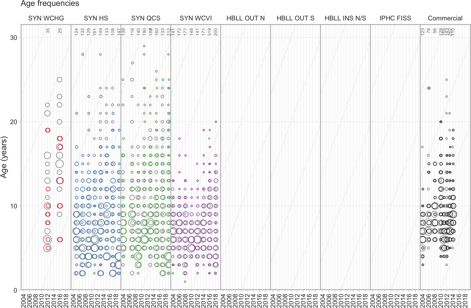
Example age-frequency plot for Petrale Sole. Female fish are shown as coloured (or black) circles and male fish are shown behind as light grey circles. The total number of fish aged for a given survey and year are indicated along the top of the panels. Diagonal lines are shown at five-year intervals to facilitate tracing cohorts through time. We plot the most recent 15 year window for which ageing data exist. See Figure 3 for survey abbreviations. Ageing precision plots comparing precision of readings by two individuals ageing the fish are provided for all species for which age data exist in Appendix A in Anderson et al. (2019).

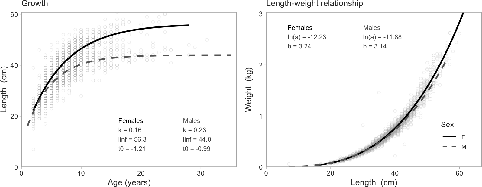
Example length-age and length-weight model fits and plots for Petrale Sole. The length-age growth curve is a von Bertalanffy model of the form Lᵢ ∼ Log-normal (log(l∞ (1 − exp(−k(Aᵢ − t₀)))), σ) where Lᵢ and Aᵢ represent the length and age of fish i, l∞, k, and t₀ represent the von Bertalanffy growth parameters, and σ represents the scale parameter. The length-weight curve is of the form log(Wᵢ) ∼ Student-t (df = 3, log(a) + b log(Lᵢ), σ), with Wᵢ and Lᵢ representing the weight and length for fish i and σ representing the observation error scale. The degrees of freedom of the Student-t distribution is set to 3 to be robust to outliers. The variables a and b represent the estimated length-weight parameters.

Female model fits are indicated as solid black lines and male model fits are indicated as dashed grey lines. Text on the panels shows the parameter estimates and open grey circles represent individual fish that the models are fit to. These figures include all survey samples. See Appendix H in Anderson et al. (2019) for details on the models.

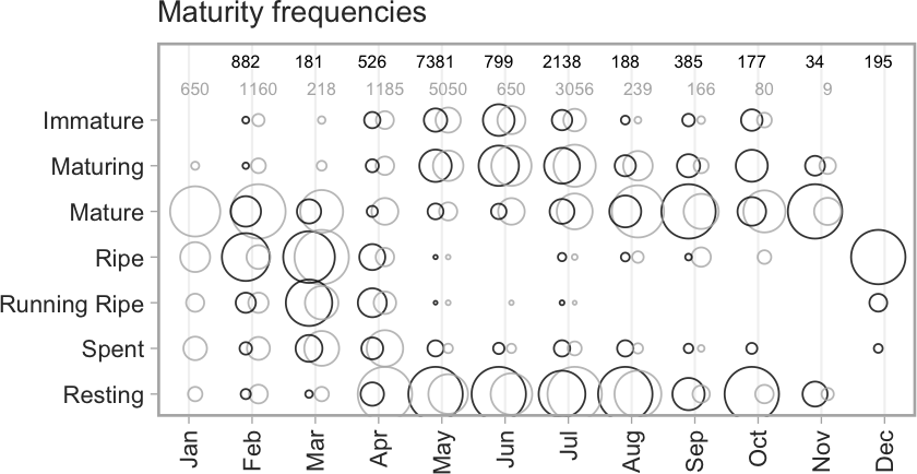
Example maturity-frequency-by-month plot for Petrale Sole. Categories of maturity are listed from most immature (top) to most mature (bottom); individual fish, once mature, cycle through the mature stages. The area of each circle corresponds to the number of fish specimens in a given maturity category for the given month. Female fish are indicated by black circles and male fish are indicated by light grey circles behind. The total number of fish specimens for each month are indicated by the numbers at the top of the plot. This plot includes data from both the commercial and survey samples.

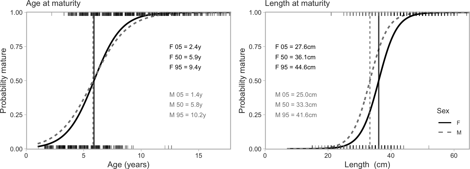
Example age- and length-at-maturity ogive plots for Petrale Sole. Maturity ogives are fit as logistic regressions to individual fish specimens, which are categorized as mature vs. not mature. The solid black lines represent fits to the female fish and the dashed grey lines represent fits to the male fish. The vertical lines indicate the estimated age or length at 50% maturity. Text on the panels indicates the estimated age and length at 5, 50 and 95% maturity for females (F) and males (M). Model fits are only shown for cases where there are at least 20 mature and 20 immature males and females. Short rug lines along the top and bottom of each panel represent up to 1500 randomly chosen individual fish with a small amount of random jittering in the case of ages to help differentiate individual fish. Models are fit to all available survey samples regardless of time of year. See Appendix H in Anderson et al. (2019) for details.